ML-Ch6-Decision Trees

Decision Trees: A Powerful Tool for Machine Learning

Decision trees are versatile machine learning algorithms that can perform both classification and regression tasks, and even multioutput tasks. They are the fundamental components of random forests, which are among the most powerful machine learning algorithms available today.

Training and Visualizing a Decision Tree

To start, we’ll train a decision tree on the well-known Iris dataset and visualize it using Graphviz.

from sklearn.datasets import load_iris
from sklearn.tree import DecisionTreeClassifier
from sklearn.tree import export_graphviz
from graphviz import Source

iris = load_iris(as_frame=True)
X_iris = iris.data[["petal length (cm)", "petal width (cm)"]].values
y_iris = iris.target

tree_clf = DecisionTreeClassifier(max_depth=2, random_state=42)
tree_clf.fit(X_iris, y_iris)

# Define file paths
dot_filename = "iris_tree.dot"
png_filename = "iris_tree"

export_graphviz(
    tree_clf,
    out_file=dot_filename,
    feature_names=["petal length (cm)", "petal width (cm)"],
    class_names=iris.target_names,
    rounded=True,
    filled=True
)

graph = Source.from_file(dot_filename)
graph.render(png_filename, format="png")

---

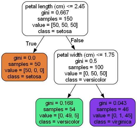
Making Predictions

One of the many qualities of decision trees is that they require very little data preparation. In fact, they don’t require feature scaling or centering at all.

Equation of Gini Impurity:

$$
Gᵢ = 1 − \sum_{k=1}^{n} (pᵢ,ₖ)^2
$$

Note: Scikit-Learn uses the CART algorithm, which produces only binary trees (trees with nodes having exactly two children). Other algorithms, like ID3, can produce trees with nodes that have more than two children.

---

Model Interpretation: White Box vs Black Box

Decision trees are intuitive and their decisions are easy to interpret. These models are often called white box models. In contrast, random forests and neural networks are generally considered black box models because their decision-making processes are harder to interpret.

The field of interpretable machine learning focuses on creating systems that can explain their decisions in a way that humans can understand. This is especially crucial in domains like healthcare and finance where fairness and accountability are paramount.

---

The CART Training Algorithm

CART (Classification and Regression Trees) works by splitting the training set into two subsets using a single feature k and a threshold $t_k$. It searches for the pair (k, $t_k$) that produces the purest subsets, weighted by their size. The algorithm then splits the subsets recursively until it reaches the maximum depth. It’s a greedy algorithm.

---

Gini Impurity vs Entropy?

Both Gini Impurity and Entropy are used to measure impurity in decision trees, but they behave slightly differently. While Gini Impurity is faster to compute, Entropy tends to produce more balanced trees.

Equation of Entropy:

$$
Hᵢ = - \sum_{k=1}^{n} pᵢₖ \log_2(pᵢₖ) \quad \text{where} \quad pᵢₖ \neq 0
$$

When to use Gini Impurity vs Entropy?

• Gini Impurity is generally faster and works well in most cases.
• Entropy tends to produce slightly more balanced trees but can be more computationally intensive.

---

Regularization Hyperparameters

• Nonparametric models: These models do not have a fixed number of parameters, so they can adapt closely to the data.
• Parametric models: Models like linear regression have predefined parameters, limiting flexibility and reducing overfitting risk.
• Regularization: To avoid overfitting, we need to restrict the decision tree’s flexibility. One common way to do this is by limiting the depth of the tree.

---

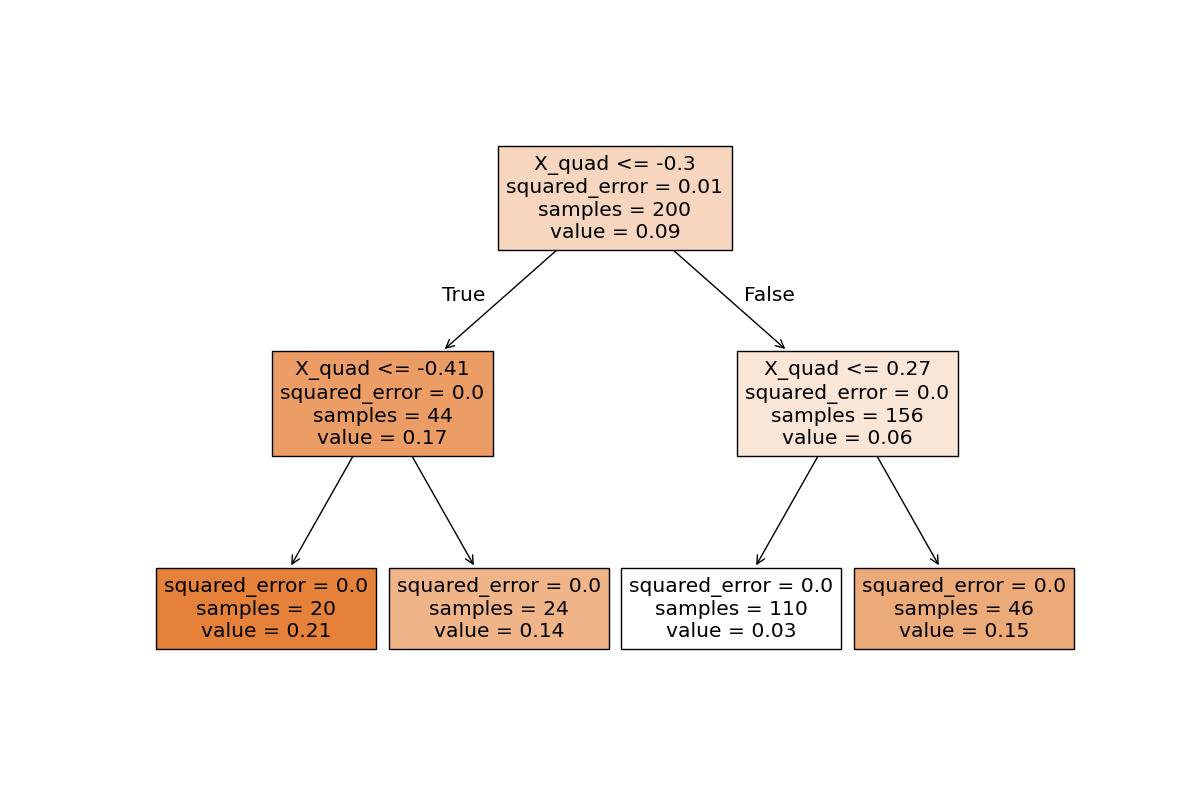
Regression with Decision Trees

Decision trees are also capable of performing regression tasks. Here’s how you can train a decision tree regressor using a quadratic dataset:

import numpy as np
from sklearn.tree import DecisionTreeRegressor

np.random.seed(42)
X_quad = np.random.rand(200, 1) - 0.5  # a single random input feature
y_quad = X_quad ** 2 + 0.025 * np.random.randn(200, 1)

tree_reg = DecisionTreeRegressor(max_depth=2, random_state=42)
tree_reg.fit(X_quad, y_quad)

from sklearn.tree import plot_tree
import matplotlib.pyplot as plt

plt.figure(figsize=(12,8))
plot_tree(tree_reg, filled=True, feature_names=["X_quad"], precision=2)
plt.show()

---

Decision Trees Have a High Variance

The main challenge with decision trees is their high variance. Small changes to the hyperparameters or the data can produce significantly different models. To mitigate this, we can average predictions over many trees, as done in Random Forests.

A random forest is an ensemble of decision trees that reduces variance and is one of the most powerful machine learning models available today.